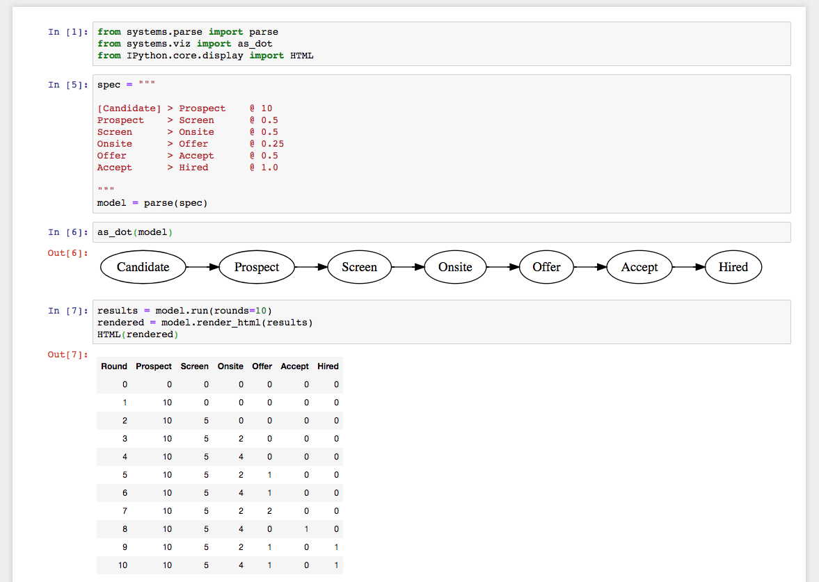
System dynamics in a jupyter notebook.

A few weeks ago I published version 0.0.1 of the systems library, and today I cut 0.0.2, which was pretty much exclusively focused on making it work better in a jupyter notebook workflow, which is still one of the best tools I’ve ever found for iterative exploration.

This post walks through the steps to get systems running in a Jupyter notebook. (You can see the final notebook on Github as well.

Installation and setup

The first step is getting Jupyter and systems installed:

mkdir jupyter
cd jupyter
python3 -m venv ./env
source ./env/bin/activate
pip install jupyter systems

Now that you’ve got that installed, you can run create a notebook via:

jupyter notebook

That should open a new tab in your browser pointing at your Jupyter notebooks, but you can also go there via localhost:8888/tree.

Then go ahead and create a new notebook, giving it a reasonable name, maybe systems exploration or some such.

As a final step, verify that installation worked properly by writing this code into the first section.

from systems.parse import parse
from systems.viz import as_dot
from IPython.core.display import HTML

Then run the code by clocking the Run button (this might take a while if this is the first time you’re running Jupyter. If it doesn’t work, look at the terminal where you ran jupyter notebook earlier for error messages, and you’ll have to debug that before moving forward.

For example, on my computer I have to upgrade prompt_tookit before moving forward, but prompt that wouldn’t be the case for most folks.

pip install --upgrade prompt_toolkit

Assuming you’ve gotten things working, next step is to start iterating on a model.

Creating a model

The example I’ll use here is the same one from an early post on developing a hiring funnel, since the goal is to showcase using jupyter.

Your notebook’s first cell should be importing the various dependencies:

from systems.parse import parse
from systems.viz import as_dot
from IPython.core.display import HTML

Then your second cell should include a multi-line string that includes your model and parsing the model. In theory you can split the definition and the parsing into separate cells, but I think combining them is better because it’ll ensure you immediately get errors if you accidentally specify a specification with some problems.

spec = """
[Candidate] > Recruiters(3, 7) @ 1
[Candidate] > Prospect         @ Recruiters * 3
Prospect    > Screen           @ 0.5
Screen      > Onsite           @ 0.5
# yeah and some more, eliding for example
"""
model = parse(spec)

Then you can render the model as a diagram:

as_dot(model)

For larger systems, You can change left-to-right rendering to top-to-bottom via:

as_dot(model, rankdir="TB")

And you can run the model and show the results as an inlined HTML table:

results = model.run(rounds=10)
rendered = model.render_html(results)
HTML(rendered)

With those pieces put together, you’re good! You can start iterating as you like.

What about charts?

If you want to chart your outputs, that’s pretty doable. Here’s a quick example using bokeh. First, you’ll need to install bokeh:

pip install bokeh

Then you’ll need to restart your kernel, either using the Kernel menu in your notebook, or by terminating the notebook process and starting it again. Then create a new cell with some additional imports and configuration:

from bokeh.plotting import figure, output_notebook, show
output_notebook()

Then you can render a line like this:

col = "Offer"
x = list(range(len(results)))
y = [row[col] for row in results]
p = figure(title=col)
p.line(x, y)
show(p)

This is going to output something quite simple, but you can work through the Bokeh documentation if you want to do something more interesting!

You can see the full example notebook on Github.