Modeling driving onboarding.
The How should you adopt LLMs? strategy explores how Theoretical Ride Sharing might adopt LLMs. It builds on several models, the first is about LLMs impact on Developer Experience. The second model, documented here, looks at whether LLMs might improve a core product and business problem: maximizing active drivers on their ridesharing platform.
In this chapter, we’ll cover:
- Where the model of ridesharing drivers identifies opportunities for LLMs
- How the model was sketched and developed using lethain/systems package on Github
- Exercising this model to learn from it
Let’s get started.
This is a chapter from Crafting Engineering Strategy.
Learnings
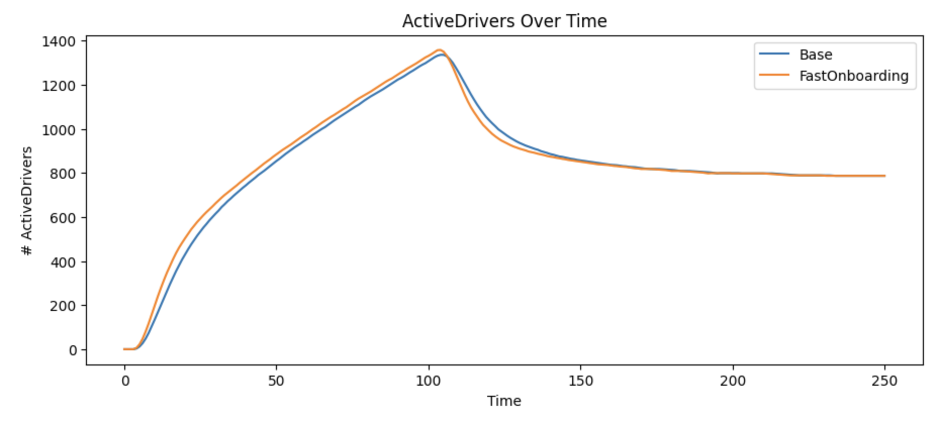
An obvious assumption is making driver onboarding faster would increase the long-term number of drivers in a market. However, this model shows that even doubling the rate that we qualify applicant drivers as eligible has little impact on active drivers over time.
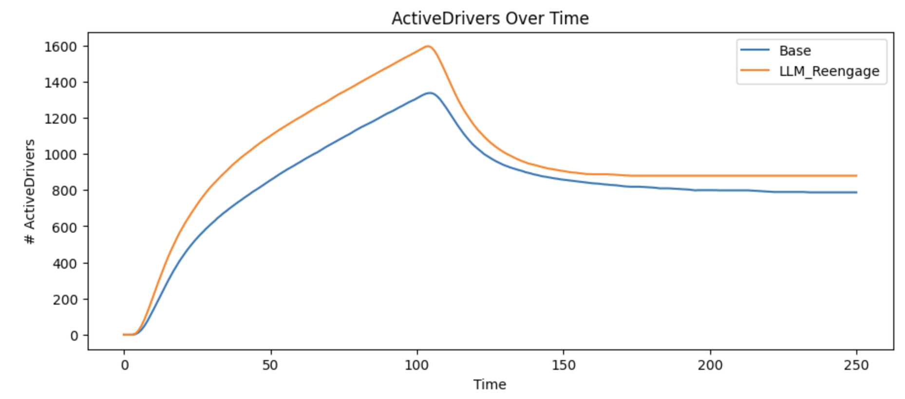
Conversely, it’s clear that efforts to reengage departed drivers has a significant impact on active drivers. We believe that there are potential LLM applications that could encourage departed drivers to return to active driving, for example mapping their rationale for departing against our recent product changes and driver retention promotions could generate high quality, personalized emails.
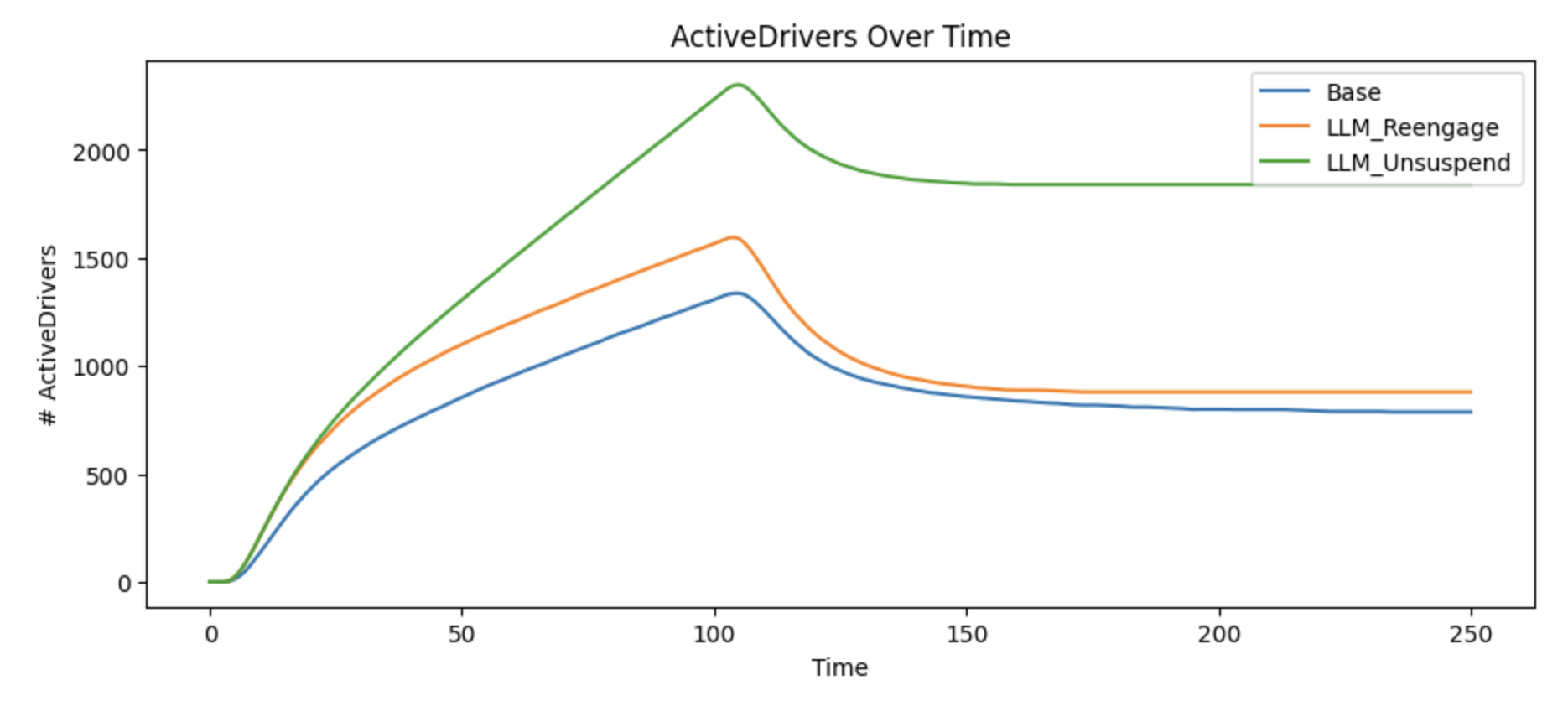
Finally, the model shows that increasing either reactivation of departed or suspended drivers is significantly less impactful than increasing both. If either rate is low, we lose an increasingly large number of drivers over time.
The only meaningful opportunities for us to increase active drivers with LLMs are improving those two reactivation rates.
Sketch
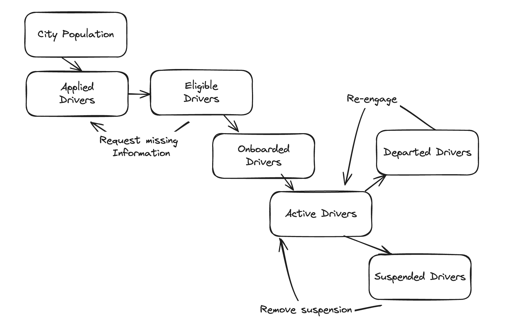
The first step in modeling a system is sketching it (using Excalidraw here). Here we’re developing a model for onboarding and retaining drivers for a ridesharing application in one city.
The stocks are:
City Populationis the total population of a cityApplied Driversare the number of people who’ve applied to be driversEligible Driversare the number of applied drivers who meet eligibility criteria (e.g. provided a current drivers license, etc)Onboarded Driversare eligible drivers who have successfully gone through an onboarding programActive Driversare onboarded drivers who are actually performing trips on a weekly basisDeparted Driverswere active drivers, but voluntarily stopped performing trips (e.g. took a different job)Suspended Driverswere active drivers, but involuntarily stopped performing trips (e.g. are no longer allowed to drive on platform)
Looking at the left-to-right flows, there is a flow from each of those stocks to the following stock in the pipeline.
These are all simple one-to-one flows, with the exception of those coming from
Active Drivers leads to two distinct stocks: Departed Drivers and Suspended Drivers.
These represent voluntary and involuntary departures.
There are a handful of right-to-left, exception path flows to consider as well:
Request missing informationrepresents a driver who can’t be moved fromApplied DriverstoEligible Driversbecause their provided information proved insufficient in a review processRe-engagetracksDeparted Driverswho have decided to start driving again, perhaps because of a bonus program for drivers who start driving againRemove suspensionrefers to drivers who were involuntarily removed, but who are now allowed to return to driving
This is a fairly basic model, but let’s see what we can learn from it.
Reason
Now that we’ve sketched the system, we can start thinking about which flows are going to have the largest impact, and where an LLM might increase those flows. Some observations from reasoning about it:
- If a city’s population is infinite, then what really matters in this model is how many new drivers we can encourage to join the system. On the other hand, if a city’s population is finite, then onboarding new drivers will be essential in the early stages of coming online in any particular city, but long-term reengaging departed drivers is probably at least as important.
- LLMs tooling could speed up validating eligible drivers. If we speed that process up enough,
we could greatly reduce the rate of the
Request missing informationflow by identifying missing information in real-time rather than requiring a human to review the information later. - We could potentially develop LLM tooling to craft personalized messaging to
Departed Drivers, that explains which of our changes since their departure might be most relevant to their reasons for stopping. This could increase the rate of theRe-engageflow - While we likely wouldn’t want an LLM approving the removal of suspensions, we could have it look at requests to be revalidated, and identify promising requests to focus human attention on the highest potential for approval.
- We could build LLM-powered tooling that helps a city resident decide whether they should apply to become a driver by answering questions they might have.
As we exercise the model later, we know that our assumptions about whether this city has already exhausted potential drivers will quickly steer us towards a specific subset of these potential options. If all potential drivers are already tapped, only work to reactivate prior drivers that will matter. If there are more potential drivers, then likely activating them will be a better focus.
Model
For this model, we’ll be modeling it using the lethain/systems library that I wrote.
For a more detailed introduction, I recommend working through the tutorial in the repository,
but I’ll introduce the basics here as well.
While systems is far from a perfect tool, as you experiment with different modeling techniques
like spreadsheet-based modeling and SageModeler,
I think this approach’s emphasis on rapid development and reproducible, sharable models is somewhat unique.
If you want to see the finished model, you can find the model and visualizations in the Jupyterhub notebook in lethain:eng-strategy-models. Here we’ll work through the steps behind implementing that model.
We’ll start by creating a stock for the city’s population, with an initial size of 10,000.
# City population is 10,000
CityPop(10000)
Next, we want to initialize the applied drivers stock, and specify a constant rate of 100 people in the city applying to become drivers each round. This will only happen until the 10,000 potential drivers in the city are exhausted, at which point there will be no one left to apply.
# 100 folks apply to become drivers per round
# the @ 100 format is called a "rate" flow
CityPop > AppliedDrivers @ 100
Now we want to initialize the eligible drivers stock, and specify that 25% of the folks in applied drivers will advance to become eligible each round.
Before we used @ 100 to specify a fixed rate.
Here we’re using @ Leak(0.25) to specify the idea
of 25% of the folks in applied drivers advancing into eligible driver.
# 25% of applied drivers become eligible each round
AppliedDrivers > EligibleDrivers @ Leak(0.25)
You could write this as @ 0.25, but you’d actually get different behavior,
That’s because @ 0.25 is actually short-hand for @ Conversion(0.25),
which is similar to a leak but destroys the unconverted portion.
Using an example to show the difference, let’s imagine that we have 100 applied drivers and 100 eligible drivers, and then see the consequences of applying a leak versus a conversion:
Leak(0.25)would end with 75 applied drivers and 125 eligible driversConversion(0.25)would end with 0 applied drivers and 125 eligible drivers
Depending on what you are modeling, you might need leaks, conversions or both.
Moving on, next we model out first right-to-left flow. Specifically, the request missing information flow where some eligible drivers end up not being eligible because they need to provide more information.
# This is "Request missing information", with 10%
# of folks moving backwards each round
EligibleDrivers > AppliedDrivers @ Leak(0.1)
Note that the syntax for left-to-right and right-to-left flows is identical, without making a distinction.
Now, 25% of eligible drivers become onboarded drivers each round.
# 25% of eligible drivers onboard each round
EligibleDrivers > OnboardedDrivers @ Leak(0.25)
Then 50% of onboarded drivers become active drivers, actually providing rides.
# 50% of onboarded drivers become active
OnboardedDrivers > ActiveDrivers @ Leak(0.50)
The active drivers stock is drained by two flows: drivers who voluntarily depart become departed drivers, and drivers who are suspended become suspended drivers. Both flows take 10% of active drivers each round.
# 10% of active drivers depart voluntarily and involuntarily
ActiveDrivers > DepartedDrivers @ Leak(0.10)
ActiveDrivers > SuspendedDrivers @ Leak(0.10)
Finally, we also see 5% of departed drivers returning to driving each round. Similarly, we unsuspend 1% of suspended drivers.
# 5% of DepartedDrivers become active
DepartedDrivers > ActiveDrivers @ Leak(0.05)
# 1% of SuspendedDrivers are reactivated
SuspendedDrivers > ActiveDrivers @ Leak(0.01)
We already sketched this model out earlier, but it’s worth noting
that systems will allow you to export models via Graphviz.
These diagrams are generally harder to read than a custom drawn one,
but it’s certainly possible to use this toolchain to combine sketching
and modeling into a single step.

Now that we have the model, we can get to exercise it to learn its secrets.
Exercise
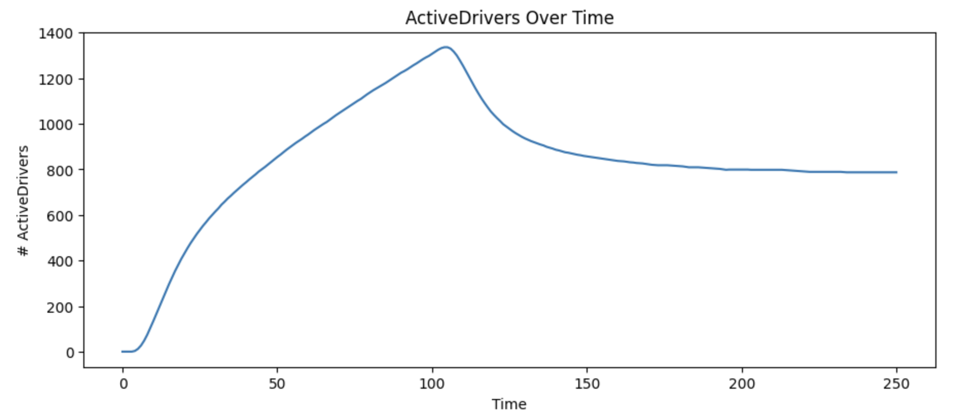
Our base model acquires initial drivers quickly, then slows as city population is exhausted.
Now let’s imagine that our LLM-powered tool can speed up eligible drivers, doubling the speed that we move applied drivers to eligible drivers. Instead of 25% of applied drivers becoming eligible each round, we’ll instead see 50%.
# old
AppliedDrivers > EligibleDrivers @ Leak(0.25)

# new
AppliedDrivers > EligibleDrivers @ Leak(0.50)
Unfortunately, we can see that even doubling the speed at which we’re onboarding drivers to eligible has a minimal impact.

To finish testing this hypothesis, we can eliminate the Request missing information flow entirely
and see if this changes things meaningfully, commenting out that line.
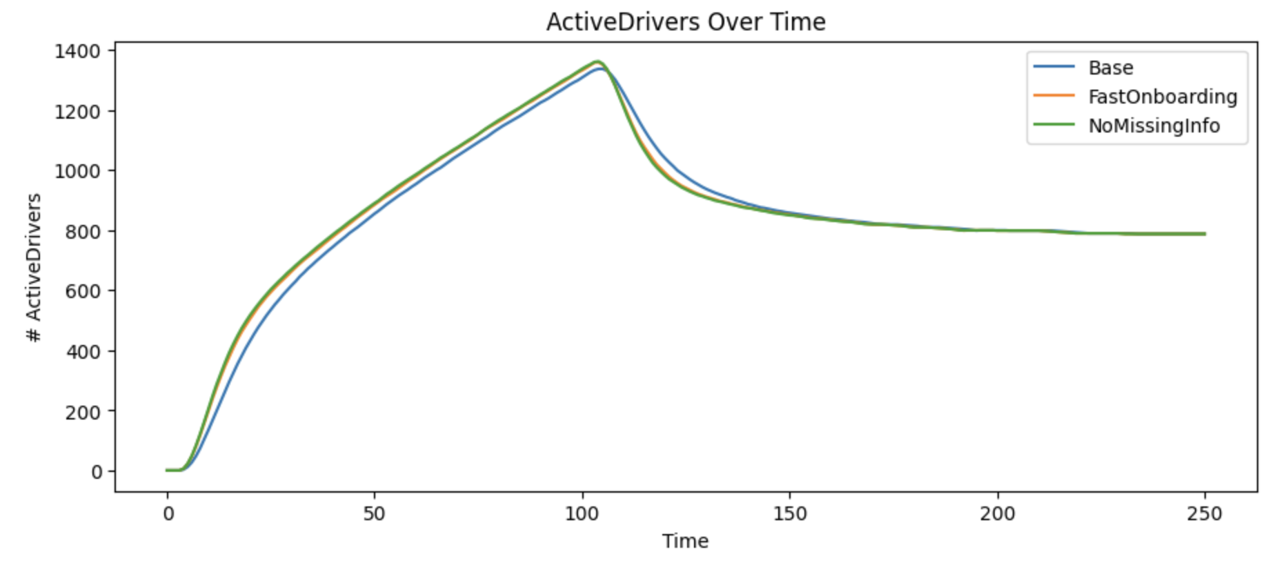
Unfortunately, even eliminating the missing information rate has little impact on the number of active drivers. So it seems like the opportunity for our LLM solutions to increase active drivers are going to need to focus on reactivating existing drivers.
Specifically, let’s go from 5% of departed drivers reactivating to 20%.
# 20% of DepartedDrivers become active
# DepartedDrivers > ActiveDrivers @ Leak(0.05)
# DepartedDrivers > ActiveDrivers @ Leak(0.2)
For the first time, we’re seeing a significant shift in impact. We reach a much higher percentage of drivers at peak, and even after we exhaust all drivers in a city, the total number of active reaches a higher equilibrium.

Presumably increasing the rate that we reactivate suspended drivers from 1% to 2.5% would have a similar, meaningful but smaller impact on active drivers over time. So let’s model that change.
# 2.5% of SuspendedDrivers are reactivated
#SuspendedDrivers > ActiveDrivers @ Leak(0.01)
SuspendedDrivers > ActiveDrivers @ Leak(0.025)
However, surprisingly, the impact of increasing the reactivation rate of suspended drivers is actually much higher than reengaging departed drivers.

This is an interesting, and somewhat counter-intuitive result. Increasing the rate for both suspended and departed rates is more impactful than increasing either, because ultimately there’s a growing population of drivers in the slower deflating stock. This means, surprisingly, that a tool that helps us quickly determine which drivers could be unsuspended might matter more than the small size of the flow indicates.
At this point, we’ve probably found the primary story that this model wants to tell us: we should focus efforts on reactivating departed and suspended drivers. Changes elsewhere might reduce operational costs of our business, but they won’t solve the problem of increasing active drivers.